Simulation Method
The COVID-19 Outbreak Simulator simulates the spread of SARS-CoV-2 virus in population as follows:
- Population: A group of individuals in a population in which everyone is susceptible. The population can be divided into multiple subgroups with different parameters such as infectivity and susceptibility.
- Introduction of virus: One or more virus carriers can be introduced to the population at the beginning of the simulation, after a period of self-quarantine, or during the simulation (community infection). The introduction of virus can happen once or multiple times.
- Spread of virus: Infected individual might or might not show symptoms (asymptomatic cases), and have varying probability to infect others (determined by a random production number). The infectees are chosen by random although individuals can have different “vicinity” and some groupss can be more or less susceptible. Infection events are pre-simulated but may not actually happen if the virus carrier is quarantined or removed, or if the infectee has already been inected.
- Handling of infected individuals: Individuals are by default removed from from the population (separated, quarantined, hospitalized, or deceased, as long as he or she can no longer infect others) after they show symptoms, but options are provided to act otherwise (e.g. quarantine after testing positive).
- End of simulation: The simulation is by default stops after the population is free of virus (all infected individuals have been removed), or everyone is infected, or after a pre-specified time (e.g. after 10 days).
- Output of simulation: The simulator outputs all events (see Output from the simulator for details) such as infection and quarantine. A summary report is generated to summarize these events. Further analysis could be performed on both the raw log file and summary report.
Limitations of the simulator
- The simulator does not simulate “contact” or “geographic locations”. Although it has a ceonvept of vicinity, it can only simulate scenrios when each group is well-mixed and have the same probability of being infected.
Concepts
-
Infectivity is modeled as the cummulative transmissibility of an infected individual during the course of infection, and is controlled by parameters
symptomatic_r0andasymptomatic_r0. For example, if one individual is symptomatic and hassympatomatc_r0=2, then he will on average infect two people. The time that the carrier will infect others will be simulated according to transmissibility distributions when an infected becomes infected. -
Vicinity determines the number of surrounding individuals from different groups, and is determined by parameter
vicinity. Vivinity only specifies sizes, not physical locations, so this parameter only impact probabilities of being infected. For example, if an individual is from groupAwith--vicinity A-B=50, he will be able to infect everyone from groupAand50individuals from groupB. Similarly,--vicinity A-B=0will make individuals from group A only infect another individual from groupA(if there are only two groups), and--vicinity A-A=5 A-B=10basically says anyone fromAwill be twice more likely to infect someone from groupB. -
susceptibility determine how likely the individual who are selected will actually become infected, which can be used to simulate level of self-protection. For example, in a population with
doctorsandpatients,doctorsmight be less susceptibility due to higher level of awareness and protection, although they may have a lot higher numbers of attempted infections. -
incubation period is the time before a symptomatic carrier shows symptom. This has nothing to do with transmissibility because asympatomatic and presympatomatic carriers can infect others.
-
leadtime is used to determine at which stage an individual in his or her course of infection when he is introduced to the population.
leadtime=anymeans any time,leadtime=asymptomaticmeans anytime before incuration period for sympatomatic carriers, or anytime for asymptomatic carriers. -
interval of simulation determines the time scale of simulation, which is by default
1/24meaning that all events can happen at each hour.
Statistical models
We developed multiple statistical models to model the incubation time, serial interval, generation time, proportion of asymptomatic transmissions, using results from multiple publications. We validated the models with empirical data to ensure they generate, for example, correct distributions of serial intervals and proporitons of asymptomatic, pre-symptomatic, and symptomatic cases. The models will continuously be updated as we learn more about the epidemiological features of COVID-19.
Assumptions
Basic assumptions,
- A distribution of incubation period (before symptoms appear) with a mean of 5.1 days and range from 2 to 11 days.
- A reproduction number $R_0$ between 1.4 and 2.8, which is the expected number of individuals the carrier will infect if he or she is not removed from the population in a population in which everyone is susceptible at probability 1 (infection will always succeed). Note that $R_0$ is not a fixed number and is the average number of a population. It will vary from population to population, and over time with changing parameters such as social distancing.
- Asymptomatic carrier will not show symptom throughout their course of infection, but their infectiousness (transmissibility) would be much smaller than symptomatic carriers.
Infection process: Infectivity, vicinity, and susceptibility
Infection is simulated in covid10-outbreak-simulator as follows:
- An individual is infected, by another carrier from the population or by community infection.
- The infectee is randomly determined to be symptomatic or asymptomatic dependening on parameter
prop-asym-carriers - An R0 value is drawn from
symptomatic-r0orasymptomatic-r0, from which zero or more infection events will be scheduled. - At the time of infection, a groups of potential infectees will be selected according
to parameter
vicinity, and an individual will be randomly selected as the infectee. If the carrier is quarantined or removed, no one will be chosen so the infection will fail. - If the selected indivdiual is not fully suscepbible (determined by parameter
susceptibility), a random number will be used to determine if he will be infected. If the infectee was infected before, he or she will not be infected again. Otherwise, infection will be successful and trigger more infection events.
An INFECTION event can trigger the following events:
- No infection will happen if at the time of infection the infector (carrier) is quarantined
or removed. In this case an
INFECTION_AVOIDEDevent will be recorded. - An infectee is randomly chosen but he or she has an
susceptibilityvalue less than 1, and is randomly determined to be not infected. In this case anINFECTION_FAILEDevent will be registered. Another rarer case ofINFECTION_FAILEDis when no one is available to be infected. - An infectee is randomly chosen, but he or she has already been infected before. In this
case and
INFECTION_IGNOREDevent will be recorded. - If the selected individual is infected, an
INFECTIONevent will happen and trigger the next infection process.
Therefore, whereas symptomatic_r0 and asymptomatic_r0 determines the average number of
infectees during the course of infection, the actual number of infectees is affected by many
factors such as quarantine, testing, population seroprevalence, and is usually lower.
Distribution of incubation period
According to Lauer et al. and their later update, estimated median incubation time (IT) of COVID-19 was 5.1 days; mean IT was 5.5 days. For 97.5% of infected persons, symptoms appear by 11.5 days. Fewer than 2.5% are symptomatic within 2.2 days. Estimated median IT to fever was 5.7 days. This estimate has been used by a recent Science paper.
According to this reference, the distribution could be modeled by different distributions, with small differences in the shape of distribution. The authors chose to use a lognormal model with parameters 1.621 and 0.418. The 2.5%, 50%, and 97.5% quantile for incubation time are 2.2, 5.05, and 11.5 days, respectively.
import numpy as np

incubation_period = np.random.lognormal(mean=1.621, sigma=0.418, size=10000)
np.quantile(incubation_period, q=[0.025, 0.5, 0.975])
array([ 2.22814544, 5.02558832, 11.4157195 ])
%get incubation_period
library(repr)

options(repr.plot.width=6, repr.plot.height=4)

hist(incubation_period, xlab='incubation period',
    main=paste('Histogram of incubation period (mean=',
              round(mean(incubation_period), 1), ')'))

Serial interval
Serial interval is defined as the days between the primary case (infector) developing symptoms and secondary case (infectee) developing symptoms. According to Nishiura et al, the mean serial interval for COVID-19 is 4.6 days with confidence interval between 3.5 and 5.9 days. These estimates agree largely with results from other sources such as Du et al, which reported that the mean interval was 3.96 days (95% CI 3.53–4.39 days), SD 4.75 days (95% CI 4.46–5.07 days); 12.6% of case reports indicated presymptomatic transmission.
Negative serial intervals were observed for COVID-19, meaning that the infectee developed symptoms before the infector, supporting the role of pre-symptomatic transmission.
We use the distributions of serial intervals to validate our models because serial intervals are combined results of incubation and virus transmission.
Du et al used a distribution of N(3.96, 4.75), with (3.53, 4.39) as the 95% CI for mean, and (4.46, 5.07) as the 95% CI for standard deviation. This distribution is more realistic than the lognormal models used by other authors, who followed the traditional assumpion of positive serial intervals.
Data from Du et al has 12.6% cases of negative serial intervals, which is less than the 20% percent of negative intervals as N(3.86, 4.75) indicates. We will use both quantities to validate our results.
from scipy.stats import norm

# quantiles
serial_intervals = np.random.normal(loc=3.96, scale=4.75, size=10000)
np.quantile(serial_intervals, q=[0.025, 0.5, 0.975])
array([-5.45908985, 3.98873037, 13.33131496])
# percent of negative serial intervals
norm(3.96, 4.75).cdf(0)
0.2022294789782194
%get serial_intervals

hist(serial_intervals, xlab='Serial intervals',
    main=paste('Histogram of serial intervals (mean=',
              round(mean(serial_intervals), 1), ')'))

Asymptomatic transmission
According to recent studies, asymptomatic transmission, names transmissions from virus carriers who will never show any symptom or show only mild symptoms that perhaps resemble allergy, plays a non-significant, but non-negligible role in the transmission of COVID-19 virus (reports). Although true asymptomatic transmissions have been identified (e.g. Bai et al, Mizumoto et al), most patients who carried the virus and showed no symptom during testing showed symptoms after a while (75% in a week). The proportion of “true” asymptomatic carriers was reported to be 17.9% from the Diamond Pincess cruise ship Mizumoto et al, 25% as estimated by CDC, and 40% from a recent mathematical model published in Science (Ferretti et al).
The infectiousness of these asymptomatic carriers are estimated to be much lower than symptomatic carriers. Liu et al. reported that the mean viral load of severe cases was around 60 times higher than that of mild cases, suggesting that higher viral loads might be associated with severe clinical outcomes. Mild cases were found to have an early viral clearance, with 90% of these patients repeatedly testing negative on RT-PCR by day 10 post-onset. By contrast, all severe cases still tested positive at or beyond day 10 post-onset. Ferretti et al models the relative infectiousness of asymptomatic infectors is 1/10 of symptomatic infectors. With an extremely high percentage of asymptomatic cases (40%) in that model, about 6% of all infectees were estimated to be infected by asymptomatic carriers. This number has not been confirmed by any other studies.
Because of the proportions of asymptomatic carriers are largely unknown and tend to change from population to population, we will assume the proportion of asymptomatic carriers follow a random distribution with mean of 25%, and a 95% confidence interval between 10% and 40%.
Generation time
The generation time is defined for source-recipient transmission pairs as the time between the infection of the source and the infection of the recipient. Because serial interval equals ($t_2$ + $i_2$) - ($t_1$ + $i_1$) = ($t_2$ - $t_1$) + ($i_2$ - $i_1$) = generation time + ($i_2$ - $i_1$) where $t$ and $i$ are infection and incubation times, generation time are usually estimated from serial interval, but should be always positive and have smaller variance.
Ferretti et al chose to estimate generation time directly and modeled the distribution of generation time with Weibull distribution with mean and median equal to 5.0 days and standard deviation of 1.9 days. The estimated mean generation time is larger than mean serial number (~4.0 days) reported elsewhere so we will compare but will not try to adjust our simulations to match the estimated distribution.
Distribution of generation time, according to Table 1 of Ferretti et al follows a Weibull distribution with parameters (2.826 and 5.665)
gt = 5.665 * np.random.weibull(2.826, 10000)
%get gt
hist(gt, main=paste0('Distribution of Generation Time (mean=', round(mean(gt), 1),
                     ", sd=", round(sd(gt), 1), ')'), xlab='Days')

Proportions of asymptomatic, pre-symptomatic and sympatomatic transmissions
Ferretti et al have also estimated the fraction of pre-symptomatic, symptomatic, environmental, and asymptomatic infections to be 47%, 38%, 10%, and 6% respectively (table 2), with the assumption of 40% of virus carriers will not show any symptom. Our model does not consider environmental infections because environmental exposures on a FPSO vessel is expected to be much lower than in a more open environment. We aim to provide realistic proportions of asymptomatic and pre-symptomatic transmissions because symptomatic individuals are promptly removed from the environment..
Modeling Transmissibility
-
For each replicated simulation, we allow a proportion of asymptomatic infectors. The proportion ranges from 10% to 40% following a random distribution centered at 25%.
-
Asymptomatic infectors will not show any symptom. They will have an overall production number ranging from
0.28to0.56, in contrast to1.4to2.8for symptomatic transmissions. This 5 fold reduction is smaller than the 10 fold reduction suggested by Ferretti et al but we believe that the gap between asymptomatic and symptomatic infectors should be smaller and should be even modeled with a continuous distribution for the two cases because the line between asymptomatic and symptomatic infectors can be quite blurred and there is no justification for the gap of $R_0$. -
According to various reports (CDC, ScienceAlert, and a study on Singapore cases), people infected and experience no symptoms or very mild symptoms may have very high viral load for the first few days, and that most presymptomatic transmission exposure occurred one to three days before a person developed symptoms. We therefore shifted the peak of the transmissbility distribution to 2/3 of the incubation date.
import numpy as np
from scipy.optimize import bisect
from scipy.stats import norm
def rand_incu(size=1):
    return np.random.lognormal(mean=1.621, sigma=0.418, size=size)
sd_6 = bisect(lambda x: norm.cdf(14, loc=6, scale=x) - 0.975, a=0.001, b=5)

def TransProb(incu, R0, interval=1/24):
    '''Transmission probability.
    incu
        incubation period in days (can be float)

    R0
        reproductive number, which is the expected number of infectees

    interval
        interval of simulation, default to 1/24, which is by hours

    returns

      x
          time point
      y
          probability of transmission for each time point
    '''
    # right side with 6 day interval
    incu = incu * 2 / 3
    dist_right = norm(incu, sd_6)
    # left hand side with a incu day interval
    sd_left = bisect(lambda x: norm.cdf(2*incu, loc=incu, scale=x) - 0.99, a=0.001, b=15, xtol=0.001)
    dist_left = norm(incu, sd_left)
    scale = dist_right.pdf(incu) / dist_left.pdf(incu)
    x = np.linspace(0, incu + 10, int((incu+10)/interval))
    idx = int(incu / interval)
    y = np.concatenate([dist_left.pdf(x[:idx])*scale, dist_right.pdf(x[idx:])])
    sum_y = sum(y)
    return x, y / sum(y) * R0
sd_5 = bisect(lambda x: norm.cdf(10, loc=5, scale=x) - 0.995, a=0.001, b=5)

def AsympTransProb(R0, interval=1/24):
    '''Asymptomatic Transmission probability.
    R0
        reproductive number, which is the expected number of infectees

    interval
        interval of simulation, default to 1/24, which is by hours

    returns

      x
          time point
      y
          probability of transmission for each time point
    '''
    dist = norm(4.8, sd_5)
    x = np.linspace(0, 12, int(12/interval))
    y = dist.pdf(x)
    sum_y = sum(y)
    return x, y / sum(y) * R0
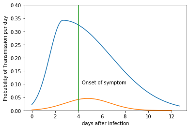
For example, if the incubation period of a carrier is 4 days, and $R_0$=2.2, the probability of transmission for each day is shown below (in blue). A similar curve for asymptomatic transmission with $R_0$=0.22 is also plotted (in orange). The distribution of asymptomatic transmission has a normal distribution centered at 5 days.
%matplotlib inline
import matplotlib.pyplot as plt

x, y = TransProb(4.0, 2.2)
x1, y1 = AsympTransProb(0.22)
plt.plot(x, y*24)
plt.plot(x1, y1*24)
plt.plot([4, 4], [0, 0.40])
plt.text(4.3, 0.10, 'Onset of symptom')
plt.ylim(0, 0.4)
plt.xlabel('days after infection')
plt.ylabel('Probability of Transmission per day')
plt.show()
Model validation
We simulated 10000 replicates of the transmissibility of an individual using the following scenario:
- Incubationn periods drawn from a log normal distribution
- $R_0$ dawn from a uniform distributed from 1.4 to 2.8
For every simulation,
- The transmission probability is calculated as described above
- A binomial distribution is applied at each hour to simulate the transmission of virus to another person. Overall number of infectees are recorded.
- Incubation periods of infectees are drawn from the same log normal distribution
- Serial intervals are calculated as the symptom date between the infector and infectee
def Infect(incu, R0, interval=1/24):
    if incu == -1:
        # asymptomatic
        x, p = AsympTransProb(R0, interval)
    else:
        x, p = TransProb(incu, R0, interval)
    infected = np.random.binomial(1, p, len(x))
    if incu == -1:
        asymptomatic_infected = sum(infected)
        presymptomatic_infected = 0
        symptomatic_infected = 0
    else:
        asymptomatic_infected = 0
        presymptomatic_infected = len([xx for xx, ii in zip(x, infected) if ii and xx < incu])
        symptomatic_infected = len([xx for xx, ii in zip(x, infected) if ii and xx >=incu])
    n_infected = sum(infected)
    if n_infected > 0:
        first = list(infected).index(1)*interval
        if np.random.uniform(0, 1) < 0.25:
            # new case is asymptomatic
            si = -99
        elif incu == -1:
            # old case is asymptomatic
            si = -99
        else:
            symp = first + rand_incu()[0]
            si = symp - incu
        return n_infected, asymptomatic_infected, presymptomatic_infected, symptomatic_infected, si, first
    else:
        return 0, 0, 0, 0, -99, 0
N = 100000

P_asym = 0.25

N_asymptomatic = int(N*P_asym)
N_regular = N - N_asymptomatic

incubation_period = np.concatenate([rand_incu(size=N_regular), np.full(N_asymptomatic, -1)])
R0 =  np.concatenate([np.random.uniform(1.4, 2.8, size=N_regular),
                      np.random.uniform(1.4/5, 2.8/5, size=N_asymptomatic)])


all_r0 = []
all_r = []
all_r_asym = []
all_r_presym = []
all_r_sym = []
all_si = []
all_gt = []
for incu, r0 in zip(incubation_period, R0):
    all_r0.append(f'{round(r0, 1):.1f}')
    r, r_asym, r_presym, r_sym, si, gt = Infect(incu, r0)
    all_r.append(r)
    all_r_asym.append(r_asym)
    all_r_presym.append(r_presym)
    all_r_sym.append(r_sym)
    all_si.append(si)
    all_gt.append(gt)
%get all_r0 all_r all_r_asym all_r_presym all_r_sym all_si all_gt
all_r = as.numeric(all_r)
all_r_asym = as.numeric(all_r_asym)
all_r_presym = as.numeric(all_r_presym)
all_r_sym = as.numeric(all_r_sym)
all_si = as.numeric(all_si)
all_gt = as.numeric(all_gt)
The following table shows the mean number of asymptomatic, presymptomatic, and symptomatic production numbers for different $R_0$ values. The rows with $R_0<0$ are rows with asymptomatic transmissions.
library(plyr)
library(dplyr)
df=data.frame(R0=as.factor(all_r0), r=all_r, r_asym=all_r_asym,
              r_presym=all_r_presym, r_sym=all_r_sym, si=all_si, gt=all_gt)
ddply(df, .(R0), function(x)
      { c(mean_r0 = mean(x$r),
        mean_r_asym=mean(x$r_asym),
        mean_r_presym=mean(x$r_presym),
        mean_r_sym=mean(x$r_sym)
        )})
| R0 | mean_r0 | mean_r_asym | mean_r_presym | mean_r_sym |
|---|---|---|---|---|
| <fct> | <dbl> | <dbl> | <dbl> | <dbl> |
| 0.3 | 0.3114241 | 0.3114241 | 0.0000000 | 0.0000000 |
| 0.4 | 0.4109496 | 0.4109496 | 0.0000000 | 0.0000000 |
| 0.5 | 0.4994408 | 0.4994408 | 0.0000000 | 0.0000000 |
| 0.6 | 0.5462963 | 0.5462963 | 0.0000000 | 0.0000000 |
| 1.4 | 1.4075691 | 0.0000000 | 0.7045124 | 0.7030568 |
| 1.5 | 1.4730740 | 0.0000000 | 0.7636500 | 0.7094241 |
| 1.6 | 1.5893382 | 0.0000000 | 0.8180147 | 0.7713235 |
| 1.7 | 1.6594393 | 0.0000000 | 0.8407477 | 0.8186916 |
| 1.8 | 1.8183161 | 0.0000000 | 0.9697194 | 0.8485968 |
| 1.9 | 1.8901515 | 0.0000000 | 0.9469697 | 0.9431818 |
| 2.0 | 2.0218291 | 0.0000000 | 1.0308619 | 0.9909673 |
| 2.1 | 2.1191537 | 0.0000000 | 1.0645880 | 1.0545657 |
| 2.2 | 2.2261458 | 0.0000000 | 1.1487603 | 1.0773854 |
| 2.3 | 2.3358321 | 0.0000000 | 1.1585457 | 1.1772864 |
| 2.4 | 2.3687110 | 0.0000000 | 1.2240176 | 1.1446934 |
| 2.5 | 2.5116014 | 0.0000000 | 1.3039178 | 1.2076835 |
| 2.6 | 2.5620357 | 0.0000000 | 1.2834324 | 1.2786033 |
| 2.7 | 2.6849262 | 0.0000000 | 1.3663559 | 1.3185703 |
| 2.8 | 2.8368794 | 0.0000000 | 1.4950355 | 1.3418440 |
Generation time is only available for simulations with at least one infectee. The distributio of generation time generally decreased with incraese produciton time ($R_0$), and have a overall mean of 4.1 and standard devitation of 2.5.
all_row = dim(df)[1]
df_r = df[df$r > 0, ]
row_with_r = dim(df_r)[1]
options(repr.plot.width=6, repr.plot.height=4)

ddply(df_r, .(R0), function(x)
      { c(
        mean_gt=mean(x$gt),
        sd_gt=sd(x$gt)
        )})

hist(df_r$gt, xlab='Days', main=paste0("Generation time ( ", round(row_with_r/all_row*100, 1),
           "% of simulations): mean=", round(mean(df$gt), 1), " std=", round(sd(df$gt),1), ")\n"))
| R0 | mean_gt | sd_gt |
|---|---|---|
| <fct> | <dbl> | <dbl> |
| 0.3 | 4.603998 | 1.907061 |
| 0.4 | 4.627946 | 1.863005 |
| 0.5 | 4.570048 | 1.913478 |
| 0.6 | 4.284923 | 1.966402 |
| 1.4 | 4.490594 | 2.716685 |
| 1.5 | 4.445273 | 2.754045 |
| 1.6 | 4.495428 | 2.651129 |
| 1.7 | 4.307651 | 2.632217 |
| 1.8 | 4.155815 | 2.629038 |
| 1.9 | 4.216110 | 2.583221 |
| 2.0 | 4.107953 | 2.594372 |
| 2.1 | 4.075569 | 2.554676 |
| 2.2 | 4.014748 | 2.531489 |
| 2.3 | 3.910110 | 2.437691 |
| 2.4 | 3.932872 | 2.475258 |
| 2.5 | 3.853754 | 2.428909 |
| 2.6 | 3.805522 | 2.425377 |
| 2.7 | 3.802404 | 2.465587 |
| 2.8 | 3.663207 | 2.322715 |

The distribution of serial intervals has a mean of 4.1 days and standard deviation of 3.7 days. There are overall 12% of negative serial intervals, which agrees well with observed cases.
library(plyr)
library(dplyr)

df_si = df_r[df_r$si != -99, ]
row_with_si = dim(df_si)[1]

ddply(df_si, .(R0), function(x)
      { c(mean_si = mean(x$si),
        std_si=sd(x$si),
        prec_neg=sum(x$si < 0)/length(x$si)
        )})

hist(df_si$si, xlab='Days', main=paste0("Serial interval ( ", round(row_with_si/all_row*100, 1),
           "% of cases): N(", round(mean(df_si$si), 1), ", ", round(sd(df_si$si),1),
                                       "), neg=",  round(sum(df_si$si<0)*100/row_with_si,1), "%\n"))
| R0 | mean_si | std_si | prec_neg |
|---|---|---|---|
| <fct> | <dbl> | <dbl> | <dbl> |
| 1.4 | 4.546973 | 3.764258 | 0.09068323 |
| 1.5 | 4.420089 | 3.738917 | 0.09003215 |
| 1.6 | 4.510535 | 3.820499 | 0.09944410 |
| 1.7 | 4.252373 | 3.796522 | 0.11000622 |
| 1.8 | 4.059037 | 3.643867 | 0.10248987 |
| 1.9 | 4.253474 | 3.708581 | 0.10193004 |
| 2.0 | 4.185517 | 3.648288 | 0.10229885 |
| 2.1 | 4.159789 | 3.778120 | 0.11585366 |
| 2.2 | 4.122831 | 3.722660 | 0.10136674 |
| 2.3 | 4.006130 | 3.575783 | 0.10207515 |
| 2.4 | 3.801754 | 3.680192 | 0.12240553 |
| 2.5 | 3.786357 | 3.550409 | 0.11936194 |
| 2.6 | 3.836003 | 3.642260 | 0.13490364 |
| 2.7 | 3.698731 | 3.665226 | 0.13351955 |
| 2.8 | 3.674834 | 3.723582 | 0.13796576 |

The overall proportion of asyptomatic, pre-symptomatic and symptomatic infections are 6%, 48% and 46%, which agrees with Ferretti et al (6% pre-symptomatic, 47% pre-symptomatic, 38% symptomatic) since this model does not consider environmental infection (16%).
ra = sum(df$r_asym)
rp = sum(df$r_presym)
rs = sum(df$r_sym)
ra / (rp + rs + ra)
rp / (rp + rs + ra)
rs / (rp + rs + ra)
0.0628321536664998
0.479099640142037
0.458068206191463